Hello and welcome to our new blog in which we discuss how to use pivot table in excel, Have you ever wondered how to get insights into your data? As there are many tools out there like Qlike View, Power BI, Jmpo, Booby A, etc, But they are very complex. They’re usually expensive and takes a lot of time to learn.
That’s when you should think of pivot tables in Excel. Because it is very easy to implement immediately, with no extra cost, because you already might have Excel. So pivot table is an Excel feature, which is a very powerful feature for data analysis by and the end of this article you’ll be able to learn how to develop your tables for your own data.
What is Pivot Table
A pivot table is a feature of Excel that is helpful to summarize, analyze, explore, and present data. It’s an interactive way to quickly summarize a large amount of data. Another hand, your charts, complement your tables were adding visualizations to the summary of data to a table and that’s going to easily see comparisons patterns and trends. The Pivot table and chart inform you to make a decision about critical data.
When to use pivot table
A pivot table can be used when you’re creating a large amount of data in many ways. For example, subtotaling and aggregating data summarizing data by categories and subcategories, and creating custom calculations from loss. Also used for filtering, sorting, and grouping of data.
Data Set for this Demo
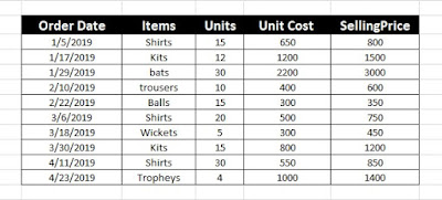
For demo purposes, we use the sales order data of a sports shop, as you see here this data has the order date on which the order took place. The items that were ordered and how many units of the item that was ordered and the cost of each unit. And at the same time the price to which we are going to sell.
Data Setup and cleaning
When you have data make sure that it is in tabular form as shown here and make sure that it doesn’t have any blank and empty values and it is correctly formatted. So that it is easy for us to make a proper analysis if there are any spaces you can turn those off using functions but usually making sure that everything is in simple table form will help. Basically, we have to do data clean-up before we start using this data for our data analysis.
How to use pivot table in excel
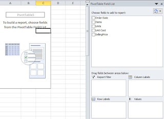
Your table can be created very easily as you look at this data just click on one of these cells and go to the insert tab and here you can see the options of the pivot table. Click the pivot table as you see here a new small pop-up form and it has two options, new worksheets, and existing worksheets.
So basically, it is asking, Where you want to place this new pivot table that is going to be created. Just select the default value and click OK. As soon as you click OK, you can see your pivot table area got created here on the left side. And on the right side, we have a new panel which has a bunch of features in it just drag and drop any items into the below fields, that your new table is formed that’s how you created your table.
How to use pivot table fields
On the other hand side of the panel, has multiple sections in it. The first section shows all the list of fields your data has, and we have four different sections that can be used to arrange the data according to you. So basically, you just have to drag and drop these columns into one of these four sections to get the results you want. It basically depends on what kind of analysis you want to do, is it row-wise or columns-wise. You can use the corner field, to sum up, your data. Apply filter of your own choice. For example, if you want to know how many sales made in each month and for each product that means the product needs to be in the column section which is nothing but an item here and the order date will be in the row section.
How to use formulas on values in pivot table
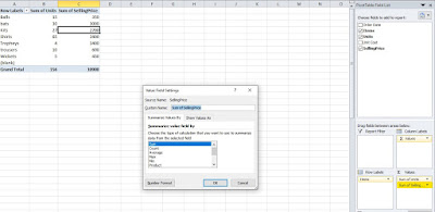
At the right bottom, you can see the section of values. If you select one of the units and click on value field settings. You can see different functions available like average, count, max, min, etc. So in this context some of the prices make sense but if you want to use the count function or any other function you just click on it and it will apply to the required column. The sum is set as the default function. If you look at these values stop showing as average or some of the units now it is being shown as a count it is very helpful to see how each item is contributing to the total sum of units.
How to use grouping in pivot table
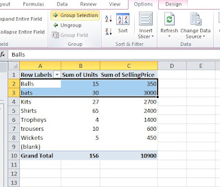
If I want to group and I choose an item like bats and balls. Simply select all those things and go to analyze and click on group selection, so you know this all formed a group now we can see how much these two items sell versus each other individual this is similar to what we have seen in the custom item here.
How to use pivot chart from the pivot table
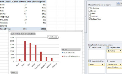
Simply go to the analyze section and click on pivot charts once you click you can select different types of charts that you want to see let’s say in this case I want to see a bar chart or column chart and click OK so now we can see that you know how many revenue or sakes take place of which item. If you want a different chart you can simply right-click and change the chart type to any other chart type depends on how you want to see.

